This lab uses a small combinational circuit to illustrate certain aspect of SystemVerilog using software available from Altera. If you would like a more detailed example using finite state machines, try out Altera’s Using ModelSim to Simulate Logic Circuits in Verilog Designs. Be sure to download the example programs first.
You can also find a pretty good overview of Verilog in the Verilog overview & references page at Texas A&M.
Creating a ModelSim project
Go to the command line and execute the following commands to start up ModelSim.
mkdir -p csci/255/svlab
/opt/altera/15.0/modelsim_ase/bin/vsim &
In the ModelSim program, use the menu choices
File ⇒
New ⇒
Project.
Next use
/home/username/csci/255/svlab,
where username is your login name,
as the Project Location
and use
svlab as the
Project Name.
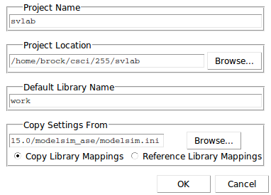
Next, you’ll see a little window.
Press Create New File.
Create a file with the name
fulladder.sv
and the type of SystemVerilog
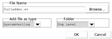
You can now close the dialog box for adding more items to the project.
Go back go the command line, type the following command to make sure you have files in the right place. You should see six files or directories.
ls -lR ~/csci/255
Completing the SystemVerilog program
Under the Project tab, double-click on fulladder.sv . This will allow you to start editing your program
You won’t get much help from ModelSim in getting started, so insert the following as your SystemVerilog program.
// CSCI 255 lab

module fulladder(
   input logic An,          // A bit
   input logic Bn,          // B bit
   input logic Cn,          // carry-in bit
   output logic Cnp1,       // carry-out bit
   output logic Sn) ;       // sum bit

   // your implementation will go here

endmodule
All the modifications you do to this program will be made
between the module header and
and the endmodule keyword.
Notice that SystemVerilog doesn’t use as many braces as C and Java. It is a bit old fashioned.
In this lab are going to implement a full-adder circuit. You can find a detailed description of the full-adder circuit in Circuits Today. You can also find an interesting picture of one on Discovery magazine.
A structural implementation
In SystemVerilog the wire is a path for connecting modules.
Add a declaration for the three wires.
wire tAB, tAC, tBC ;
Now implement your module by placing the
the following structural description after the wire
declaration.
All your inputs, outputs and wires are now used in your program.
      xor(Sn, An, Bn, Cn) ;
      and(tAB, An, Bn) ;
      and(tAC, An, Cn) ;
      and(tBC, Bn, Cn) ;
      or(Cnp1, tAB, tAB, tBC) ;
The and, or and xor are some
of the predefined gates that are provided by SystemVerilog.
If you want to name your gates, you can use the following syntax.
      xor  sum(Sn, An, Bn, Cn) ;
      and  abTerm(tAB, An, Bn) ;
      and  acTerm(tAC, An, Cn) ;
      and  bdTerm(tBC, Bn, Cn) ;
      or   carry(Cnp1, tAB, tAC, tBC) ;
Go ahead compile your module with Compile ⇒ Compile All. The result of the compile will appear in the Transcript window. If there are errors, you will need to use View ⇒ Message View window to uncover the messages.
Simulation of the full adder
Text-based simulation
Press
Simulate ⇒
Start Simulation.
This will raise the
Start Simulation window,
where you must expand the work library to
select the fulladder module.
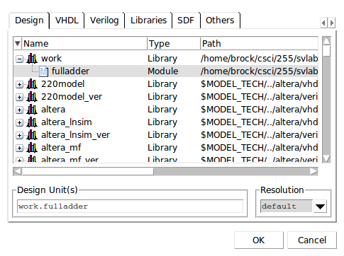
Afterwards, there will be a flurry of flashing windows.
Take a minute to look at these windows. The Transcript window is the console for a TCL program that controls the simulation. In the real world, designers write TCL scripts to customize the simulation.
In the Objects window,
notice the values of your variables.
For now, consider HiZ and StX
to be uninitialized values.
In the Transcript window, issue the following commands.
force An 0
force Bn 0
force Cn 0
run 100
This will initialize An, Bn and
Cn and
“run” your
circuit for 100 picoseconds.
You should see that all you variables now have the value
St0, a strong 0.
Now set An to 1 and run for another 100.
The values of An and Sn should change.
All those buttons
It is possible to use all those buttons to simulate your program. You can run your mouse slowly over the buttons or you can read the Altera tutorial or you can just keep typing commands.
Riding the wave
Use your mouse to select the five input and output values of your circuit. Right-click and use Add to ⇒ Wave ⇒ Selected Signals to add these values to the wave display.
You can always mash Simulate ⇒ Run ⇒ Restart to reinitialize the simulation if things look weird, but then you will then toforce all your variables.
Set An back to 0 and run another 100.
You should now see your values displayed on the wave.
Let’s to go through all eight combinations of the input using a Gray code. Use these 16 commands to do the checking. Each time you type run 100, make sure the outputs look correct.
force Cn 1
run 100
force Bn 1
run 100
force Cn 0
run 100
force An 1
run 100
force Cn 1
run 100
force Bn 0
run 100
force Cn 0
run 100
force An 0
run 100
Kind of tedious, ain’t it? Go ahead and stop the simulation with Simulate ⇒ End Simulation, and we’ll try something better.
A testbench program
Let’s add a testbench module to the project The testbench module will not be synthesized. It is purely for debugging.
You’ll need to create a new file. Select the Project tab and follow that with Project ⇒ Add to Project ⇒ New File. Name the new file testbench.sv and make sure it is of type SystemVerilog. It will not be added to the library until it is successfully compiled.
In this section of the lab, you will modify only the testbench module.
Do not modify the fulladder module.
SystemVerilog without a circuit
Here is the code for the testbench module.
This looks a lot like a C or Java loop to print
from 0 to 7,
except that it uses begin-end rather
than curly braces to surround the body of the for.
There is also a reg declaration.
In SystemVerilog, a register is a variable for storing values.
module testbench() ;
   reg[2:0]  vin ;
   integer i ;

   initial begin
      for (i=0; i<8; i=i+1)
      begin
         vin = i ; #100 ;
         $display("vin = %h", vin) ;
      end
   end
endmodule
The #100 is SystemVerilog’s way of delaying for
100 picoseconds.
Start the simulator but choose only
testbench for the simulation.
(I had trouble seeing testbench and had to
close fulladder. Odd.)
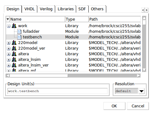
Either press the Run -All button (if you can find it) or just type run -all to start the simulation. (About the only thing the buttons do is talk to TCL.)
You should get a count from 0 to 7.
Go ahead and end the simulation and we’ll try for something a bit more useful.
Testing the full adder
Now we are going to add a “call”
of the fulladder module from the testbench.
To do this, you need a wire to connect
the output of
fulladder to the testbench.
The fulladder will be instantiated as
dut, for device under test.
This is a common naming convention in Verilog.
Place the following two
statements right before the initial begin keywords
to instantiate the fulladder and connect it to the testbench.
  wire[1:0] vout ;

  fulladder dut(vin[2], vin[1], vin[0], vout[1], vout[0]) ;
Next go into the initial begin block
and modify the call to $display so that
in prints out vout.
$display("vin = %h, vout = %h", vin, vout) ;
Compile all your programs but save them first. Start up the simulation, but select only the testbench. It will include the needed copy of the device under test.
Hopefully, you will get the right answers.
You might want to replace the %h in the call
to $display with %b to get binary output.
Back on the wave
Try out the wave simulator by adding in
vin and vout.
You will need to expand them to see the individual bits.
Testbench is complete
At this point, your work on the testbench is complete.
You should never modify the testbench module again.
A behavioral description
The structural description is a good way to match a circuit, but it doesn’t look like a program.
Go to the fulladder and comment out
the structural description. Just enclose everything from the
wire declaration to the or gate with
the usual Java/C /* and */ comment delimiters.
Now add in a simple behavioral description.
      assign Sn = An ^ Bn ^ Cn ;
      assign Cnp1 = An & Bn | An & Cn | Bn & Cn ;
Except for the assign keyword, it looks just like
C or Java. Simulate it to see that it works fine.
If you don’t like those logical C/Java operators, you can just
use the regular addition operator, but you need to add a
two-bit declaration of a variable sum2bit to do this.
     wire[1:0] sum2bit ;

     assign sum2bit = An + Bn + Cn ;
     assign Sn = sum2bit[0] ;
     assign Cnp1 = sum2bit[1] ;
Again, simulate.
Finally, you can also take advantage of Verilog’s own special use of braces to concatenate bitstrings to write a one-statement implementation.
assign {Cnp1, Sn} = An + Bn + Cn ;
And simulate one more time.
Trying out Quartus
Exit from ModelSim and start up Quartus. (It may take a while for Quartus to start.)
/opt/altera/15.0/quartus/bin/quartus &Use the menu choices File ⇒ New Project Wizard to create a Quartus project for synthesis. The project wizard will guide you through many screens.
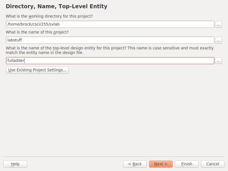
In one of the early screens,
create your project in the same directory that you used above.
and select fulladder as your top-level design entry.
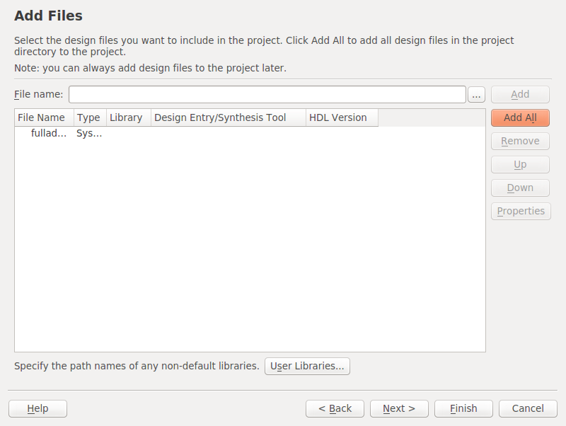
When you get to the screen to add files,
Click on the three dots just to the left of the
Add button, and
use the browser to select your
fulladder.v file.
Do not use the testbench program.
Since we don’t have any Cyclone IV’s,
just choose the first device you see, the EP4CGX15BF14A7.
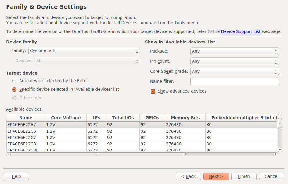
Use the defaults in the remaining screens.
With Processing ⇒ Start Compilation, you should now be able to compile and synthesize. Expect lots of warnings.
Examining the results
Now just poke around a little.
Under Assignments, look at Pin Planner. There you will see how your five pins are mapped to the pins of the Cyclone IV FPGA.
Close the Pin Planner window and return to the main Quartus window. Use Tools ⇒ Netlist Viewers ⇒ RTL Viewer to view the compilation of your SystemVerilog program to gates. Without closing the RTL Viewer window, use Tools ⇒ Netlist Viewers ⇒ Technology Map Viewer (Post Mapping) to view the compilation into the combinational logic cells of the FPGA.
The combinational logic cells are implemented by the LUT, or look-up table. The LUT is a multiplexer connected to SRAM, memory that is loaded when the FPGA is turned on. Take a look at Figure 3 on page 2 of Altera’ white paper on FPGA architecture to see how a LUT is implemented in silicon.