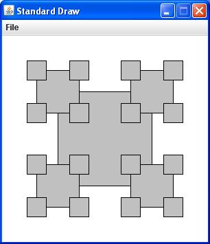
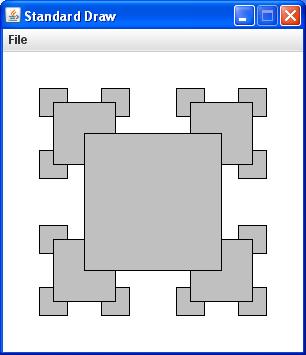
Let your MySquares program accept two command-line arguments:
- An integer n, specifying the order of the recursive plot (where n = 1 denotes a single square).
- An integer s, used to specify which of the two types of plot to render (let s = 1 and s = 2 specify the left and right plots respectively).
Now Build the project and run MySquares from the terminal window. When everything is working, show your results to your lab instructor.
When you think you understand what this program is supposed to do, open Brownian.java in the NetBeans editor and look over the source code. Your goal at this stage is to see if you can understand just how this program performs its task. And again, get help from your lab instructor as necessary.
Then Build your project again, and run this program using various values of its single command-line argument (the so-called Hurst exponent H).
The first change you want to make is based on the fact that Brownian uses recursion to break up an initially straight, horizontal line into 2n segments, where n is the order of the recursion. However, the recursive method curve() as defined in Brownian uses a base case that tests for a minimum segment length rather than the order n. This motivates your first task: revise MyBrownian.java so that it accepts the recursive order n as an additional command-line argument, and explicitly uses the value n = 0 to serve as its base case.
As your second task, have the program accept the initial variance var, aka the volatility, as a third command-line argument. This should let you confirm that the volatility affects the overall scale of the vertical displacements, whereas the Hurst exponent H affects the smoothness of the curves.
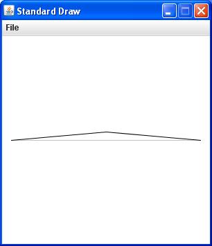
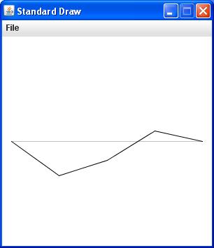
When these changes are in place, Build your Lab10 project again and run MyBrownian. If you initially fix var = 0.01 and H = 0.0 and make successive runs with n = 1 and n = 2, you should get images roughly like the ones shown below:
If you now get brave and let n = 10, you should see something more like the leftmost image below. But if you leave n = 10 and let H = 0.5, the image should resemble the one on the right:
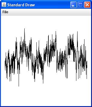
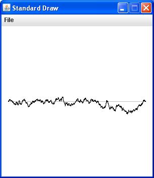
Note that this last image, where the Hurst exponent H = 0.5, is known as a Brownian bridge.
Now take a moment to try various other combinations of the three command-line arguments, and see if you understand how they affect the curves. Then show your results to your lab instructor.
As with Brownian.java, you first want to understand the purpose of PlasmaCloud.java. Infortunately, in this case neither the text (see page 272) nor the Booksite offers anything more than a sketchy discussion. You should actually get more insight by opening PlasmaCloud.java in the NetBeans editor and reading the comments as well as the source code itself. But of course, as a last resort you can always ask your lab instructor to make everything clear...
You should next run this demo a few times to get some idea of its behavior. While you are doing this, you should examine the role of the single command-line argument accepted by the current version of this program.
As you may have guessed by now, your real task here is to create a new, enhanced version of PlasmaCloud.java that might give you further insight into its behavior. You will again want to leave the original version intact for reference purposes, so first create a new copy of this demo, called (what else?) MyPlasmaCloud.java.
By this time you should realize that PlasmaCloud starts by assigning random colors (using a variant of the HSV color model) to the four corners of a unit square, and painting the entire square with an average of those four colors, or more precisely an average with an added random Gaussian fluctuation. Then it calls a recursive method that initially divides the square into four quadrants (or subsquares), and paints each quadrant with a similar average of four colors it derives for each of its corners. (These colors are themselves derived by averaging over the corner colors of the original unit square in fairly obvious ways.) And as always with recursive methods, things may not stop there...
By now you may have realized that applying this recursive process n times will break up the original unit square into 4n segments. However, the Booksite version of PlasmaCloud.java is like Brownian.java, in that it uses a base case that specifies a minimum size of the squares, rather than the minimum recursive order n. So once again your first task is to revise MyPlasmaCloud.java so that it accepts n as a command-line argument, and explicitly uses the value n = 0 to serve as its base case.
To make your second revision, locate the declaration of the variable stddev in the main() method. This quantity determines the scale of the random fluctuations in the color-averaging procedure. In the original PlasmaCloud, the value of stddev is simply assigned the value 1.0. However, the value of stddev strongly affects these images, and to understand its role here you want to convert it into a second command-line argument.
Finally, you may soon find it helpful for this program to produce smaller windows than normal. So you could optionally take care of that in main() now. But for the moment you may just want to remember that StdDraw provides this option if you need it...
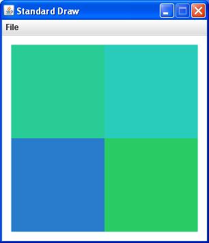
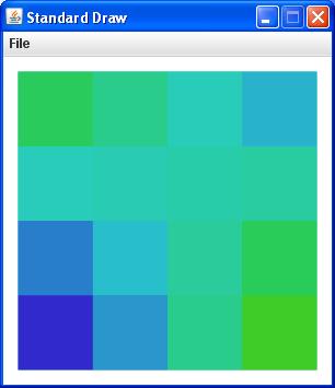
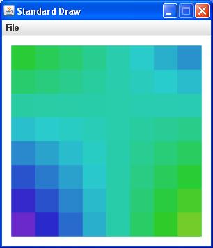
After you make these changes, Build your Lab10 project yet again and run MyPlasmaCloud. Start out by keeping stddev = 0.0 for the moment (no random fluctuations at all), and try successive runs with n = 1, n = 2, n = 3, and n = 4. Remember that your local colors will vary, but with luck you should see something like the following sequence of images:
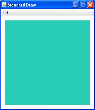
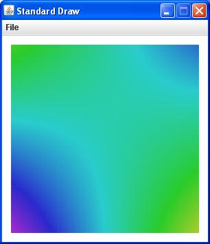
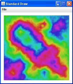
You may soon discover that things slow down fast as n increases, so you won't want to go too far with these tests. But for n = 8 and stddev = 0.0, your window might look like the leftmost image below. Of course the colors in this image change quite smoothly, since no random fluctuations have been added in the averaging procedure. However, if you keep n = 8 but now let stddev = 1.0 you might get an image more like the one on the right:
So as time permits, feel free to experiment with various values of stddev, and perhaps find other parameters to adjust in this program. But you will be officially done as soon as you can demonstrate your working version of MyPlasmaCloud to your lab instructor.