Lab 07

This lab will give you a chance to work with some examples of static methods in Java. This topic is covered in Section 2.1 of your text.

To complete this project, follow the steps listed below:

1. Login to your home directory and launch a terminal window. Use the cd command to change your default directory to csci/273/labs. Keep this window open for future reference.
2. Launch the NetBeans IDE and raise the New Project dialog. Define the project to be a Java Application named Lab07. Make sure that the project folder will be created within your csci/273/labs folder. As in your previous labs, you should also uncheck the Create Main Class checkbox before you click Finish.
3. Now download the textbook library classes StdOut.java, StdIn.java, and StdDraw.java into the default package for your project. As in Lab 05 and Lab 06, you will use these library classes without having to modify them in any way.

   Next find and download the Booksite source file Gaussian.java, which is an extended version of Program 2.1.2 in your text. In this lab you will also want to leave this program unchanged. However, you should now take a moment to look over the source code in Gaussian.java. In particular, look for two static methods named phi(). These are two versions of the Gaussian (normal) probability density function φ(x), less formally known as the bell-shaped curve, that plays a central role in statistics. This function is briefly described in Section 2.1 of your text (see pp. 193-196). As you may recall, these bell-shaped curves are characterized by the location of their peak (the mean x-value μ) and their standard deviation σ (which characterizes the width of the bell). One of the two phi() methods in Gaussian.java simply assumes that μ is 0.0 and σ is 1.0, while the other lets you provide these values as input parameters.

   You should also look for another pair of methods in Gaussian.java, which are both named Phi(). (Note the uppercase P here.) These methods both represent the Gaussian cumulative distribution function Φ(x), which is also described in your text (see above). Φ(x) gives the area under the curve φ(x'), obtained by integrating φ(x') from negative infinity to x. A plot of this curve vs. x increases monotonically from 0.0 to 1.0.

   Finally, take note of yet another pair of methods named PhiInverse(). As their name suggests, these both represent the inverse function of the cumulative distribution Φ(x). Thus PhiInverse(Phi(x)) returns x for any argument x in the domain of Φ.

   You will be working with all these functions in this lab, so you may want to look back over these method definitions as you proceed.

4. Now download two more source files into your project, this time directly from the links DrawGaussian.java and SampleGaussian.java Note that both of these files are provided by your kindly instructor, not the Booksite.
5. Build the project. This step should cause you no problems, since at this stage you are just compiling several pre-tested source files. But if anything goes wrong, check immediately with your lab instructor before proceeding.
6. Now return to your terminal window, and enter the command cd Lab07 to set your default directory to be the Lab07 project folder. As a check, use the ls dist command to list the contents of the project subfolder dist. (Note that the ls command does not change your default directory.) You should see the file Lab07.jar. If not, it's again time to consult with your lab instructor.
7. Enter the command

   
       java -cp dist/Lab07.jar DrawGaussian
       

   and you should soon see a plot of the standard Gaussian density function φ(x). Here the term standard means that the mean μ and standard deviation σ are set to 0.0 and 1.0 respectively.

   Actually, DrawGaussian lets you provide optional command-line arguments to specify the mean and standard deviation. For example, you could have produced the same plot by entering the command

   
       java -cp dist/Lab07.jar DrawGaussian 0.0 1.0
       

   Here the first command-line argument is the mean x-value μ, while the second is the standard deviation σ. Both of these are real numbers, stored as double values in the program. You should try displaying this plot several times, using different combinations of these two parameters.

   DrawGaussian actually accepts a third optional command-line argument. This one is an integer, whose default value is 1. This argument is used as a code indicating just what this program plots. For example, try entering the command

   
       java -cp dist/Lab07.jar DrawGaussian 0.0 1.0 1
       

   As you should see, the value 1 yields a plot of φ(x), like the ones you have already produced. If you change this argument to 2, you will get a plot of the cumulative distribution Φ(x) instead. You should verify this for yourself before proceeding.

   If you want to show both curves in the same plot, just change this third argument to 3. Again, try this out right away.

   Actually this third argument can be any sum of the following powers of two: (1, 2, 4). DrawGaussian is actually treating this argument as a three-bit binary switch, with each bit indicating whether to plot a particular function (1 to plot, 0 to omit).

8. So if you are really alert at the moment, you may already be wondering why the plot-code argument includes a third bit. Well, that is so you can plot the results of your next task, which is to build a histogram of x-values obtained by random sampling from the Gaussian distribution. Some of the machinery for doing this has already been written for you, in the form of the incomplete source file SampleGaussian.java which you should have downloaded earlier. So you should now open SampleGaussian.java in the NetBeans editor, and prepare to do your part...
9. Locate the method named getHistogram() in SampleGaussian. This method includes a loop over a large number of trials, where each trial consists of generating a single random value sampled from a Gaussian distribution, then binning that value into a histogram. As the comments state, your job is to complete the code in this loop, so that on each iteration the variable x actually gets a suitable random value.

   There are actually several ways to do this, and you are hereby requested to try two of them in this lab. The first algorithm is known as the Box-Muller formula, and is actually described in Exercise 1.2.27 of your text. If you do not have your text with you, you can also find the statement of this Exercise on the Booksite. So try to implement this algorithm as indicated. When you are done, Build your project again. Then return to your terminal window and enter the command

   
       java -cp dist/Lab07.jar DrawGaussian 0.0 1.0 7
       

   and show the results to your lab instructor.

   Once you have been checked out on this part, you should go back and comment out the statements in SampleGaussian.getHistogram() that you wrote based on the Box-Muller formula. (Do not actually remove them, since they may come in handy later.)

   Then replace your earlier code with statements that make use of the method PhiInverse(), which is included in the Booksite file Gaussian.java that you downloaded earlier. You will want to get help from your lab instructor on how to make use of this method here.

   When you have revised your code, Build your project yet again and show your latest results to your lab instructor.

10. As your final task in this lab, add a new Java main class to your project and use it to produce an image that looks something like the following:
    

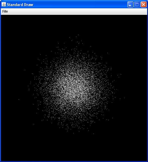
    Hint: You can generate a cluster of points like this by repeatedly sampling both x and y independently, each from a Gaussian distribution...

When your project is complete and working correctly, demonstrate it to your lab instructor. Then, before you exit NetBeans, clean your Lab07 project. Finally, before you logout, switch back to your terminal and set your default directory back to csci/273/labs. Then create a JAR file of your Lab07 project folder, using the command

jar cf Lab07Project.jar Lab07